NumPy Notes

This is the note for article A Visual Intro to NumPy and Data Representation, by Jay Alammar

Chinese version can be found at Numpy和数据展示的可视化介绍

Also, it takes some notes for another article NumPy Illustrated: The Visual Guide to NumPy, and the a Chinese version of it can be found at 图解 | NumPy可视化指南, another version is at 一图胜千言，超形象图解NumPy教程！

Big-O Cheat Sheet

Python Time Complexity

NumPy Illustrated: The Visual Guide to NumPy

1. Vectors, the 1D Arrays

初始化Numpy array用到的函数

函数	参数
`np.array(pylist)`	使用Python list来初始化一个Numpy array
`np.zeros()`	`shape, dtype=float, order='C'`
`np.ones()`	`shape, dtype=None, order='C'`
`np.empty()`	`shape, dtype=float, order='C'`
`np.full()`	`shape, fill_value, dtype=None, order='C'`
`np.zeros_like()`	`a, dtype=None, order='K', subok=True, shape=None`
`np.ones_like()`	`a, dtype=None, order='K', subok=True, shape=None`
`np.empty_like()`	`prototype, dtype=None, order='K', subok=True, shape=None`
`np.full_like()`	`a, fill_value, dtype=None, order='K', subok=True, shape=None`

使用单调序列初始化Numpy array

函数	参数
`np.arange()`	`[start,] stop[, step,], dtype=None`
`np.linspace()`	`start, stop, num=50, endpoint=True, retstep=False, dtype=None, axis=0`

创建随机数组

旧式创建方法（deprecated）

函数	参数
`np.random.randint`	`low, high=None, size=None, dtype=int`
`np.random.rand`	`d0, d1, ..., dn`
`np.random.uniform`	`low=0.0, high=1.0, size=None`

新式创建方法

首先创建对象：rng = np.random.default_rng()

函数	参数
`rng.integers`	`low, high=None, size=None, dtype=np.int64, endpoint=False`
`rng.random`	`size=None, dtype=np.float64, out=None`
`rng.uniform`	`low=0.0, high=1.0, size=None`

2. Vector indexing

基本索引操作

可以指定单个索引，索引范围，反向索引，以及数组索引

定义1D array（一维数组）

>>> a = np.arange(1, 6)
>>> a
array([1, 2, 3, 4, 5])

操作及效果

索引操作	结果	效果
`a[1]`	`2`	返回view
`a[2:4]`	`array([3, 4])`	返回view
`a[-2:]`	`array([4, 5])`	返回view
`a[::2]`	`array([1, 3, 5])`	返回view
`a[[1,3,4]]`	`array([2, 4, 5])`	fancy indexing，返回新数组

定义2D array（二维数组）

a = np.array([[3, 4, 5, 6], [2, 7, 0, -1], [1, 5, 3, 18], [2, 6, 1989, 3]])
>>> a
array([[   3,    4,    5,    6],
       [   2,    7,    0,   -1],
       [   1,    5,    3,   18],
       [   2,    6, 1989,    3]])

操作及效果

索引操作	结果	效果
`a[1]`	`array([2,7,0,-1])`	返回第`1`行
`a[2:4]`	`array([[1,5,3,18],[2,6,1989,3]])`	返回第`2`到`4`行
`a[-2:]`	`array([1,5,3,18])`	返回倒数第一行
`a[::2]`	`array([[3,4,5,6],[1,5,3,18]])`	返回第`0`和`2`行
`a[[0,1,3]]`	`array([[3,4,5,6],[2,7,0,-1],[2,6,1989,3]])`	fancy indexing，返回新数组，第`0`、`1`和`3`行
`a[:,[1,3]]`	`array([[4,6], [7,-1], [5,18], [6,3] ]])`	fancy indexing，返回新数组，第`1`和`3`列

Python list vs Numpy list

Python List	Numpy List
`a = [1, 2, 3]`	`a = np.array([1, 2, 3])`
`b = a` (no copy)	b = a (no copy)
`c = a[:]` (copy)	`c = a[:]` (no copy)
`d = a.copy()` (copy)	`d = a.copy()` (copy)

Boolean索引

定义数组：a = np.array([1, 2, 3, 4, 5, 6, 7, 6, 5, 4, 3, 2, 1])

逻辑比较（返回一个Boolean数组）

>>> a > 5
array([False, False, False, False, False,  True,  True,  True, False,
       False, False, False, False])

any和all函数

>>> np.any(a > 5)
True

>>> np.all(a > 5)
False

利用Boolean数组索引

>>> a[a > 5]
array([6, 7, 6])

>>> a[(a >= 3) & (a <= 5)]
array([3, 4, 5, 5, 4, 3])

np.where和np.clip函数

函数	参数	作用
`np.where()`	`condition, [x, y]` `condition`: array_like, bool	If `condition` is `true`, yield `x`, otherwise yield `y`. If `x` or `y` 都没有指定，返回原先数组中的值
`np.clip()`	`a, a_min, a_max, out=None, **kwargs`	指定值的范围`[a_min, a_max]`，小于`a_min`的赋值为`a_min`，大于`a_max`的赋值`a_max`

3. Vector operations

基本操作：vector之间的加减乘除整除

# 定义两个数组
>>> a = np.array([4, 8])
>>> b = np.array([2, 5])
# 加
>>> a + b
array([ 6, 13])
# 减
>>> a - b
array([2, 3])
# 乘
>>> a * b
array([ 8, 40])
# 除
>>> a / b
array([2. , 1.6])
# 整除
>>> a // b
array([2, 1], dtype=int32)
# 乘方
>>> a ** b
array([   16, 32768], dtype=int32)

基本操作：vector与scalar之间的加减乘除整除

# 定义数组
>>> c = np.array([1, 2])
# 加
>>> c + 3
array([4, 5])
# 减
>>> c - 3
array([-2, -1])
# 乘
>>> c * 3
array([3, 6])
# 除
>>> c / 3
array([0.33333333, 0.66666667])
# 整除
>>> c // 2
array([0, 1], dtype=int32)
# 乘方
>>> c ** 2
array([1, 4], dtype=int32)

截断近似函数

np.floor向下取整（round to negative infinity, -\(\infty\)）

>>> np.floor([1.1, 1.5, 1.9, 2.5])
array([1., 1., 1., 2.])

np.ceil向上取整（round to negative infinity, +\(\infty\)）

>>> np.ceil([1.1, 1.5, 1.9, 2.5])
array([2., 2., 2., 3.])

np.round向最近的整数截断（around to nearest integer）

>>> np.round([1.1, 1.5, 1.9, 2.5])
array([1., 2., 2., 2.])

一些数学函数

# 开方
>>> np.sqrt([4, 9])
array([2., 3.])
# 以e为底的幂乘
>>> np.exp([1, 2])
array([2.71828183, 7.3890561 ])
# 以e为底的对数（the logrithm of np.e to base e）
>>> np.log([np.e, np.e**2])
array([1., 2.])
# 点积
>>> np.dot([1,2], [3,4])
11
# 点积的另一种写法
>>> np.array([1,2]) @ np.array([3,4])
11
# 叉积
>>> np.cross([2, 0, 0], [0, 3, 0])
array([0, 0, 6])
# 正弦
>>> np.sin([np.pi, np.pi/2])
array([1.2246468e-16, 1.0000000e+00])
# 反正弦
>>> np.arcsin([0, 1])
array([0.        , 1.57079633])
# 平方和的开方
>>> np.hypot([3,5], [4,12])
array([ 5., 13.])

一些三角函数

三角函数	反三角函数	双曲函数	反双曲函数
`sin`	`arcsin`	`sinh`	`arcsinh`
`cos`	`arccos`	`cosh`	`arccosh`
`tan`	`arctan`	`tanh`	`arctanh`

双曲正弦函数：\(\sinh{x}\)

\[ \sinh{x} = \frac{e^x - e^{-x}}{2} \]

双曲余弦函数：\(\cosh{x}\)

\[ \cosh{x} = \frac{e^x + e^{-x}}{2} \]

双曲正切函数：\(\tanh{x}\)

\[ \tanh{x} = \frac{e^x - e^{-x}}{e^x + e^{-x}} \]

基本的统计函数

# 最大值
>>> np.max([1, 2, 3])
3
# 最大值
>>> np.array([1, 2, 3]).max()
3
# 最大值的索引
>>> np.array([1, 2, 3]).argmax()
2
# 最小值
>>> np.array([1, 2, 3]).min()
1
# 最小值的索引
>>> np.array([1, 2, 3]).argmin()
0
# 求和
>>> np.array([1, 2, 3]).sum()
6
# 求平均
>>> np.array([1, 2, 3]).mean()
2.0
# 标准差
>>> np.array([1, 2, 3]).var()
0.6666666666666666
# 方差
>>> np.array([1, 2, 3]).std()
0.816496580927726

排序函数

Python List	Numpy Arrays	Effect
`a.sort()`	`a.sort()`	sort in place
`sorted(a)`	`np.sort(a)`	return a new sorted array
`a.sort(key=f)`	-	sort with key
`a.sort(reversed=False)`	-	ascending/descending order

4. Searching for an element in a vector

Python list search - index method

Python list有index方法，而Numpy没有

a.index(x [, i [, j]])

这里x是要查找的元素，i和j分别是指定区间的上下限，如果没有找到，会raise exception

>>> a = [12, 0, -1, 78, 99]
>>> a.index(78)
3
>>> a.index(78, 4)
Traceback (most recent call last):
  File "<pyshell#6>", line 1, in <module>
    a.index(78, 4)
ValueError: 78 is not in list

Numpy list search

Numpy中有三种办法查找某个元素

np.where

>>> a = [12, 0, -1, 78, 99]
>>> np.where(a == 78)[0][0]
3

next + np.ndenumerate（这种需要Numba来加速，否则就和上面的np.where一样，比较慢）

>>> a = [12, 0, -1, 78, 99]
>>> next(i[0] for i, v in np.ndenumerate(a) if v == 78)
3

np.searchsorted

>>> a = [12, 0, -1, 78, 99]
>>> b = np.sort(a)
>>> b
array([-1,  0, 12, 78, 99])
>>> np.searchsorted(b, 78)
3

5. Comparing floats

np.allclose(a, b)用于容忍误差之内的浮点比较

but, there is no silver bullet!

表达式	结果
`0.1 + 0.2 == 0.3`	`False`
`np.allclose(0.1 + 0.2, 0.3)`	`True`
`math.isclose(0.1 + 0.2, 0.3)`	`True`

表达式	结果
`1e-9 == 2e-9`	`False`
`np.allclose(1e-9, 2e-9)`	`True`
`math.isclose(1e-9, 2e-9)`	`False`

表达式	结果
`0.1 + 0.2 - 0.3 == 0`	`True`
`np.allclose(0.1 + 0.2 - 0.3, 0)`	`True`
`math.isclose(0.1 + 0.2 - 0.3, 0)`	`False`

注意

np.allclose假定所有比较数字的尺度为1。

比如，如果在纳秒级别上，则需要将默认atol参数除以1e9：np.allclose(1e-9,2e-9, atol=1e-17)==False。
math.isclose不对要比较的数字做任何假设，而是需要用户提供一个合理的abs_tol值（np.allclose默认的atol值为1e-8）
一些问题见如下链接
- floating-point guide
- NumPy issue on GitHub.

6. Matrices, the 2D Array

基本概念

现在在Numpy中，matrix 和 2D Array 是指同一个概念，可以相互替换使用（interchangeably）
在Numpy中，原先的class matrix已经不再使用（deprecated）

定义一个Numpy 2D array：a = np.array([[1, 2, 3], [4, 5, 6]])

它的.shape属性返回一个元组，共有两个元素，第一个是行数，第二个是列数
len(a)返回的是2D array的行数

>>> a = np.array([[1, 2, 3], [4, 5, 6]])
>>> a.dtype
dtype('int32')
>>> a.shape
(2, 3)
>>> len(a)
2
>>> a.shape[0]
2

常用函数

之前的zeros，ones，full，empty还有eye都可以用来生成2D array

需要注意的是，指定2D array的元组要用括号()括起来，表示第一个参数，因为第二个参数是留给dtype的

>>> np.zeros((3, 2))
array([[0., 0.],
       [0., 0.],
       [0., 0.]])
>>> np.ones((3, 2))
array([[1., 1.],
       [1., 1.],
       [1., 1.]])
>>> np.full((3, 2), 7)
array([[7, 7],
       [7, 7],
       [7, 7]])
>>> np.empty((3, 2))
array([[1., 1.],
       [1., 1.],
       [1., 1.]])
>>> np.eye(3, 3)
array([[1., 0., 0.],
       [0., 1., 0.],
       [0., 0., 1.]])
>>> np.eye(3)
array([[1., 0., 0.],
       [0., 1., 0.],
       [0., 0., 1.]])

还有random函数

# x服从[0, 10)上的均匀分布（整数）
>>> np.random.randint(0, 10, [3, 2])
array([[7, 1],
       [6, 6],
       [2, 1]])
# x服从[0, 1)上的均匀分布
>>> np.random.rand(3, 2)
array([[0.1518058 , 0.47967987],
       [0.0242219 , 0.46161326],
       [0.64206284, 0.02072145]])
# x服从[0, 1)上的均匀分布（浮点数）
>>> np.random.uniform(1, 10, [3, 2])
array([[4.60676287, 4.64315581],
       [9.56576352, 2.2958745 ],
       [2.18304639, 5.9622002 ]])

np.random.randn，x服从标准正态分布，\( N(\mu, \sigma^2), \mu = 0, \sigma = 1 \)

# x服从标准正态分布
>>> np.random.randn(3, 2)
array([[-0.95367737, -0.35999719],
       [-0.27186541,  1.10111502],
       [-0.36303053,  0.5372727 ]])

np.random.normal，x服从正态分布，\( N(\mu, \sigma^2), \mu = 10, \sigma = 2 \)

# x服从正态分布
>>> np.random.normal(10, 2, [3, 2])
array([[10.06207497,  9.45178632],
       [ 9.02901148, 10.92862084],
       [12.53682855, 10.20647998]])

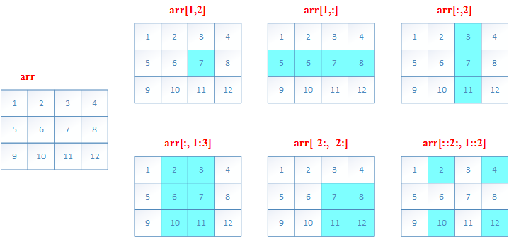
二维数组的索引（切片slice）

和一维数组的slice类似例子如下

>>> a = np.array([[1,2,3,4], [5,6,7,8], [9,10,11,12]])
>>> a[1,2]
7
>>> a[1,:]
array([5, 6, 7, 8])
>>> a[:,2]
array([ 3,  7, 11])
>>> a[:,1:3]
array([[ 2,  3],
       [ 6,  7],
       [10, 11]])
>>> a[-2:,-2:]
array([[ 7,  8],
       [11, 12]])
>>> a[::2, 1::2]
array([[ 2,  4],
       [10, 12]])

2D Array Slice

7. The axis argument

轴参数（axis argument）

Numpy引入axis参数，以便实现跨行或跨列操作
axis参数的值实际上是维度数量。（第一维axis=0，第二维axis=1，以此类推）
二维数组中，axis=0表示列方向，axis=1表示行方向

##axis	方向
`axis = 0`	列方向（即所有行）
`axis = 1`	行方向（即所有列）

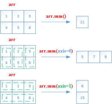
以sum为例子

>>> a = np.array([[1,2,3], [4, 5,6]])
>>> a.sum()
21
>>> a.sum(axis=0)
array([5, 7, 9])
>>> a.sum(axis=1)
array([ 6, 15])

Sum axis example

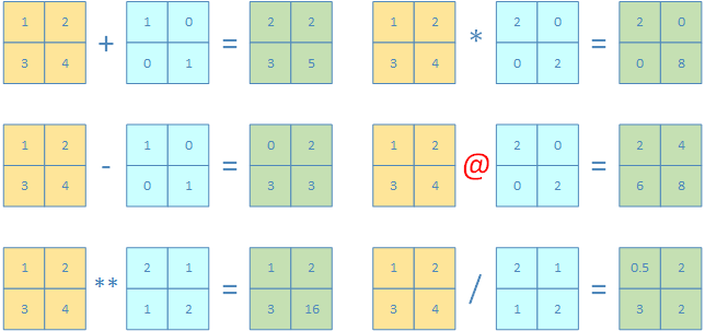
矩阵的算术运算

2D Array支持数组逐个元素之间的运算：+，-，*， /，//，**
2D Array也支持外积（outer product）

>>> np.array([[1,2],[3,4]]) + np.array([[1,0],[0,1]])
array([[2, 2],
       [3, 5]])
>>> np.array([[1,2],[3,4]]) - np.array([[1,0],[0,1]])
array([[0, 2],
       [3, 3]])
>>> np.array([[1,2],[3,4]]) ** np.array([[2,1],[1,2]])
array([[ 1,  2],
       [ 3, 16]], dtype=int32)
>>> np.array([[1,2],[3,4]]) * np.array([[2,0],[0,2]])
array([[2, 0],
       [0, 8]])
>>> np.array([[1,2],[3,4]]) @ np.array([[2,0],[0,2]])
array([[2, 4],
       [6, 8]])
>>> np.array([[1,2],[3,4]]) / np.array([[2,1],[1,2]])
array([[0.5, 2. ],
       [3. , 2. ]])

Arithmetic

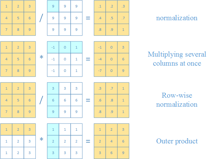
Numpy通过标量的广播机制（broadcasting from scalar），可以实现以下混合运算

向量和矩阵之间
两个向量之间

>>> a = np.array([[1,2,3], [4, 5,6], [7,8,9]])
>>> a / 9
array([[0.11111111, 0.22222222, 0.33333333],
       [0.44444444, 0.55555556, 0.66666667],
       [0.77777778, 0.88888889, 1.        ]])
>>> a * np.array([-1, 0, 1])
array([[-1,  0,  3],
       [-4,  0,  6],
       [-7,  0,  9]])
>>> a / np.array([[3],[6],[9]])
array([[0.33333333, 0.66666667, 1.        ],
       [0.66666667, 0.83333333, 1.        ],
       [0.77777778, 0.88888889, 1.        ]])
>>> np.array([1, 2, 3]) * np.array([[1], [2], [3]])		   
array([[1, 2, 3],
       [2, 4, 6],
       [3, 6, 9]])

Mixed Arithmetic

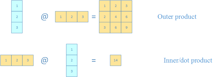
点积和叉积（内积和外积）

>>> np.array([[1],[2],[3]]) @ np.array([[1,2,3]])				   
array([[1, 2, 3],
       [2, 4, 6],
       [3, 6, 9]])

>>> np.array([1,2,3]) @ np.array([[1],[2],[3]])				   
array([14])

Inner & Outer Product

8. Row vectors & column vectors

Numpy中共有三种类型的向量

向量类型	vector types
1维数组	1D arrays
2维行向量	2D row vectors
2维列向量	2D column vectors

三种类型的vector相互之间的转换如下

Different types of vectors

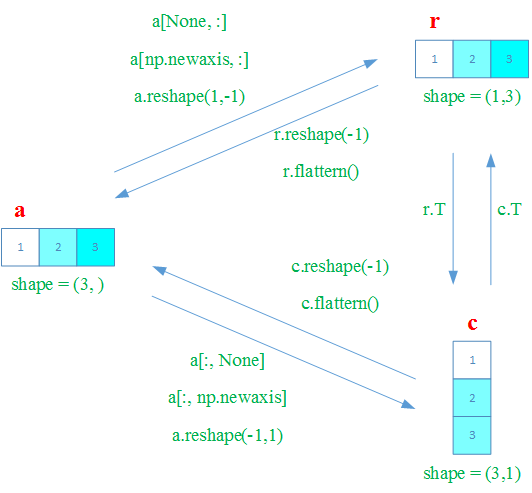
除了一维数组外，所有的数组大小（shape属性）都是一个向量
- 比如a.shape == [1, 1, 1, 5, 1, 1]
- 一维数组的大小（shape属性）是(N, )的形式
在Numpy中，一维数组默认是行向量（row vector）
注意：Numpy中，一个行向量和只有一个行向量的矩阵是不同的

一个行向量的shape属性是(n, )

需要注意的是一个行向量的转置（transpose）仍然是行向量。
```
>>> c = np.array([1, 2, 3])
>>> c.shape
(3,)
>>> c.T
array([1, 2, 3])
```
只有一个行向量的矩阵的shape属性是(1, n)

只有一个行向量的矩阵的转置（transpose）是只有一个列向量的矩阵。
```
>>> b = np.array([[1,2,3]])
>>> b.shape
(1, 3)
>>> b.T
array([[1],
       [2],
       [3]])
```
可以通过reshape把一个行向量转换为一个列向量矩阵或行向量矩阵

假定现有一个行向量a如下
```
>>> a = np.array([1, 2, 3, 4, 5, 6])
>>> a.shape
(6,)
```
转换为列向量矩阵。这里reshape的第一个参数-1表示该维度（第一个维度）上自动推断决定
```
>>> b = a.reshape(-1, 1)
>>> b
array([[1],
       [2],
       [3],
       [4],
       [5],
       [6]])
>>> b.shape
(6, 1)
```
转换为行向量矩阵。这里reshape的第二个参数-1表示该维度（第二个维度）上自动推断决定
```
>>> c = a.reshape(1, -1)
>>> c
array([[1, 2, 3, 4, 5, 6]])
>>> c.shape
(1, 6)
```

类似的，也可以使用np.newaxis来转换上面的行向量

同样的，假定现有一个行向量a如下

>>> a = np.array([1, 2, 3, 4, 5, 6])
>>> a.shape
(6,)

转换为列向量矩阵。

这里a[:, None]中的None相当于np.newaxis

>>> b = a[:, None] # 这里可以用np.newaxis替换None
>>> b
array([[1],
       [2],
       [3],
       [4],
       [5],
       [6]])
>>> b.shape
(6, 1)

转换为行向量矩阵。

>>> c = a[None, :]
>>> c
array([[1, 2, 3, 4, 5, 6]])
>>> c.shape
(1, 6)

9. Matrix manipulations

主要的函数

函数	作用
`np.hstack`	横向拼接
`np.vstatck`	纵向拼接
`np.column_statck`	用于2D和1D array横向拼接
`np.hsplit`	横向切割（沿`y`轴切割）
`np.vsplit`	纵向切割（沿`x`轴切割）
`np.tile`	2D array整体重复
`ndarray.repeat`	元素重复
`np.delete`	删除行或列
`np.insert`	插入行或列
`np.append`	可以同时实现`np.hstack`和`np.vstack`的作用
`np.pad`	在矩阵四周添加指定行数或列数的元素

拼接和分割函数

拼接函数	分割函数
`np.hstack`	`np.hsplit`
`np.vstatck`	`np.vsplit`
`np.column_statck`

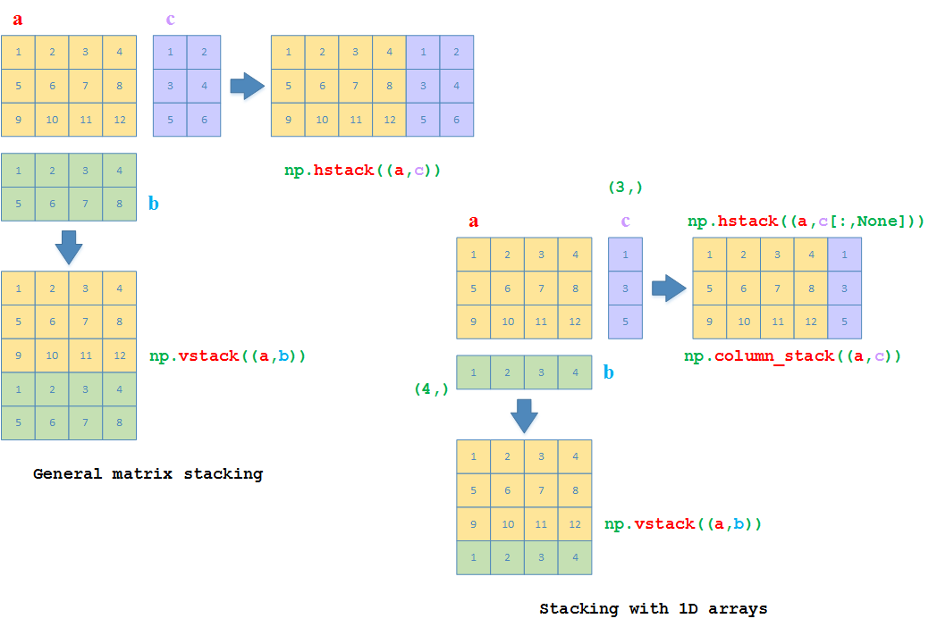
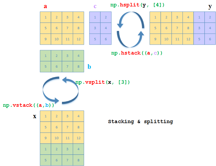
Numpy中的拼接函数

np.hstack：横向拼接
np.vstatck：纵向拼接

np.column_stack：用于2D array和1D array的横向拼接

>>> a = np.array([[1,2,3,4], [5,6,7,8], [9,10,11,12]])
>>> b = np.array([[1,2,3,4], [5,6,7,8]])
>>> c = np.array([[1,2], [3,4], [5,6]])
# 纵向拼接
>>> np.vstack((a, b))
array([[ 1,  2,  3,  4],
       [ 5,  6,  7,  8],
       [ 9, 10, 11, 12],
       [ 1,  2,  3,  4],
       [ 5,  6,  7,  8]])
# 横向拼接
>>> np.hstack((a, c))
array([[ 1,  2,  3,  4,  1,  2],
       [ 5,  6,  7,  8,  3,  4],
       [ 9, 10, 11, 12,  5,  6]])
# b和c现重新改为1D array
>>> b = np.array([1,2,3,4])
# 2D array和1D array可以直接做纵向拼接
>>> np.vstack((a, b))
array([[ 1,  2,  3,  4],
       [ 5,  6,  7,  8],
       [ 9, 10, 11, 12],
       [ 1,  2,  3,  4]])
>>> c = np.array([1,3,5])
# 2D array和1D array直接做横向拼接会抛异常
>>> np.hstack((a, c))
Traceback (most recent call last):
  File "<pyshell#10>", line 1, in <module>
    np.hstack((a, c))
  File "<__array_function__ internals>", line 6, in hstack
  File "C:\Python36\lib\site-packages\numpy\core\shape_base.py", line 346, in hstack
    return _nx.concatenate(arrs, 1)
  File "<__array_function__ internals>", line 6, in concatenate
ValueError: all the input arrays must have same number of dimensions, but the array at index 0 has 2 dimension(s) and the array at index 1 has 1 dimension(s)
# 2D array和转换为行向量的1D array再直接做横向拼接
>>> np.hstack((a, c[:,None]))
array([[ 1,  2,  3,  4,  1],
       [ 5,  6,  7,  8,  3],
       [ 9, 10, 11, 12,  5]])
# 或者直接利用np.column_stack来直接拼接2D array和1D array
>>> np.column_stack((a, c))
array([[ 1,  2,  3,  4,  1],
       [ 5,  6,  7,  8,  3],
       [ 9, 10, 11, 12,  5]])

Matrix Stacking

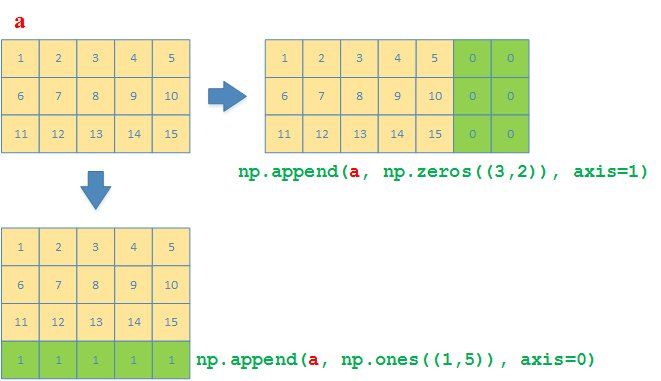
np.append函数可以同时实现np.vstack和np.hstack的效果

>>> a = np.array([[1,2,3,4,5], [6,7,8,9,10], [11,12,13,14,15]])
# 沿着y方向（列的方向），在矩阵最后添加一行，值都是1
>>> np.append(a, np.ones((1,5)), axis=0)
array([[ 1.,  2.,  3.,  4.,  5.],
       [ 6.,  7.,  8.,  9., 10.],
       [11., 12., 13., 14., 15.],
       [ 1.,  1.,  1.,  1.,  1.]])
# 沿着x方向（行的方向），在矩阵最后添加一个3x2的矩阵，值都是0
>>> np.append(a, np.zeros((3,2)), axis=1)
array([[ 1.,  2.,  3.,  4.,  5.,  0.,  0.],
       [ 6.,  7.,  8.,  9., 10.,  0.,  0.],
       [11., 12., 13., 14., 15.,  0.,  0.]])

Append rows & columns

Numpy中的分割函数

和np.vstack以及np.hstack相对应的，有分割函数

np.vsplit：沿着x轴（axis=0）进行分割（纵向分割）
- 第二个参数是行的索引（数组），表示从第几行起开始分割
- 返回一个list，某个元素是分割后的数组
np.hsplit：沿着y轴（axis=1）进行分割（横向分割）
- 第二个参数是列的索引（数组），表示从第几列起开始分割
- 返回一个list，某个元素是分割后的数组

# 纵向分割
>>> a = np.array([[1,2,3,4], [5,6,7,8], [9,10,11,12]])
>>> b = np.array([[1,2,3,4], [5,6,7,8]])
>>> x = np.vstack((a, b))
>>> np.vsplit(x, [3]) # 第二个参数是行的索引，表示从第几行起开始分割
[array([[ 1,  2,  3,  4],
       [ 5,  6,  7,  8],
       [ 9, 10, 11, 12]]),
 array([[1, 2, 3, 4],
       [5, 6, 7, 8]])]
# 横向分割
>>> a = np.array([[1,2,3,4], [5,6,7,8], [9,10,11,12]])
>>> c = np.array([[1,2], [3,4], [5,6]])
>>> y = np.hstack((a, c))
>>> np.hsplit(y, [4])  # 第二个参数是列的索引，表示从第几列起开始分割
[array([[ 1,  2,  3,  4],
       [ 5,  6,  7,  8],
       [ 9, 10, 11, 12]]),
 array([[1, 2],
       [3, 4],
       [5, 6]])]

Stacking & Splitting

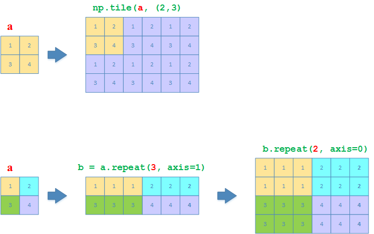
矩阵的复制

np.tile：like copy-pasting
- 相当于把整个矩阵当做一个整体，然后以该整体为单位进行复制
np.repeat：like collated printing
- 相当于对矩阵里面的每个元素，按照axist=0（列方向）或axis=1（行方向）的方式依次进行重复

>>> a = np.array([[1,2], [3,4]])
>>> np.tile(a, (2, 3))
array([[1, 2, 1, 2, 1, 2],
       [3, 4, 3, 4, 3, 4],
       [1, 2, 1, 2, 1, 2],
       [3, 4, 3, 4, 3, 4]])
>>> a.repeat(3, axis=1)
array([[1, 1, 1, 2, 2, 2],
       [3, 3, 3, 4, 4, 4]])
>>> a.repeat(3, axis=1).repeat(2, axis=0)
array([[1, 1, 1, 2, 2, 2],
       [1, 1, 1, 2, 2, 2],
       [3, 3, 3, 4, 4, 4],
       [3, 3, 3, 4, 4, 4]])

Matrix duplication

矩阵行和列的删除与插入

删除与插入函数

删除	插入
`np.delete`	`np.insert`

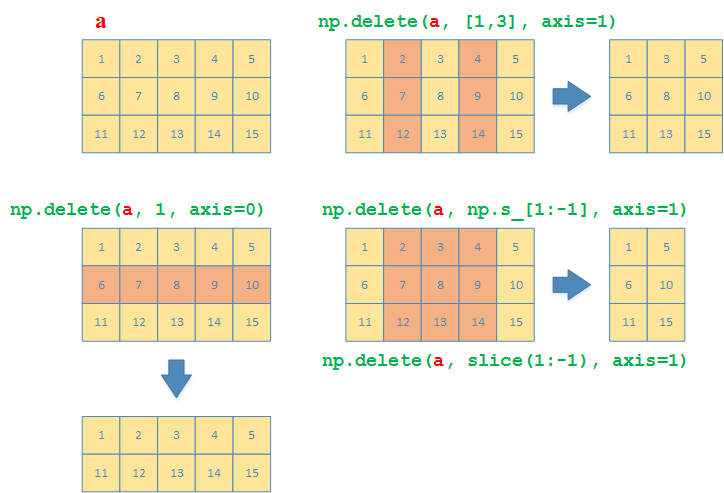
np.delete用来指定要删除的行或列，也可以同时指定多个连续或者不连续的行和列。

>>> a = np.array([[1,2,3,4,5], [6,7,8,9,10], [11,12,13,14,15]])
# 删除索引为1的行
>>> np.delete(a, 1, axis=0)
array([[ 1,  2,  3,  4,  5],
       [11, 12, 13, 14, 15]])
# 删除索引为1和3的列
>>> np.delete(a, [1,3], axis=1)
array([[ 1,  3,  5],
       [ 6,  8, 10],
       [11, 13, 15]])
# 删除第一（含）到倒数第一（不含）的列
>>> np.delete(a, np.s_[1:-1], axis=1)
array([[ 1,  5],
       [ 6, 10],
       [11, 15]])
# 删除第一（含）到倒数第一（不含）的列
>>> np.delete(a, slice(1,-1), axis=1)
array([[ 1,  5],
       [ 6, 10],
       [11, 15]])

Delete rows & columns

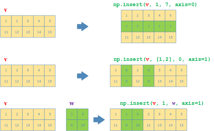
与np.delete对应的，np.insert用来指定要插入的行或列，也可以同时指定多个连续或者不连续的行和列

>>> v = np.array([[1,2,3,4,5], [6,7,8,9,10]])
# 沿着y方向（列），在第一行前面插入一行，元素都是7
>>> np.insert(v, 1, 7, axis=0)
array([[ 1,  2,  3,  4,  5],
       [ 7,  7,  7,  7,  7],
       [ 6,  7,  8,  9, 10]])
# 沿着x方向（行），在第一、二列前面分别各插入一列，元素都是0
>>> np.insert(v, [1, 2], 0, axis=1)
array([[ 1,  0,  2,  0,  3,  4,  5],
       [ 6,  0,  7,  0,  8,  9, 10]])
>>> w = np.array([[1,5], [6,10]])
# 沿着x方向（行），在第一列前面将矩阵w插入
>>> np.insert(v, [1], w, axis=1)
array([[ 1,  1,  5,  2,  3,  4,  5],
       [ 6,  6, 10,  7,  8,  9, 10]])

Insert rows & columns

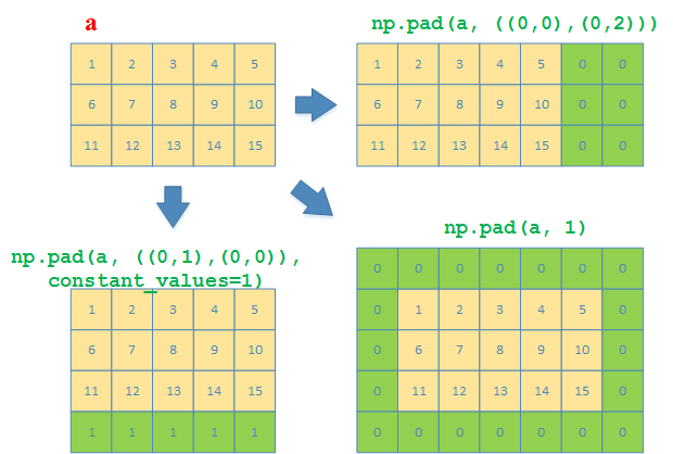
函数`pad`

在2D arrays（其实不止2D）中，np.pad可以用来给2D array（矩阵）的四周边界添加值

典型的用法比如

np.pad(arr, ((M, N), (S, T)), constant_values=1)

这里的边界参数含义如下

M：在该二维数组的第0行前面添加M行

N：在该二维数组的最后一行前面添加N行

S：在该二维数组的第0列前面添加S列

T：在该二维数组的最后一列前面添加T列

例子：

a = np.array([[1,2,3,4,5], [6,7,8,9,10], [11,12,13,14,15]])
# 在最后一行后面再添加一行
>>> np.pad(a, ((0,1),(0,0)), constant_values=1)
array([[ 1,  2,  3,  4,  5],
       [ 6,  7,  8,  9, 10],
       [11, 12, 13, 14, 15],
       [ 1,  1,  1,  1,  1]])
# 在最后一列后面再添加两列
>>> np.pad(a, ((0,0),(0,2)))
array([[ 1,  2,  3,  4,  5,  0,  0],
       [ 6,  7,  8,  9, 10,  0,  0],
       [11, 12, 13, 14, 15,  0,  0]])
# 在四周个添加一行/列
>>> np.pad(a, 1)
array([[ 0,  0,  0,  0,  0,  0,  0],
       [ 0,  1,  2,  3,  4,  5,  0],
       [ 0,  6,  7,  8,  9, 10,  0],
       [ 0, 11, 12, 13, 14, 15,  0],
       [ 0,  0,  0,  0,  0,  0,  0]])

padding

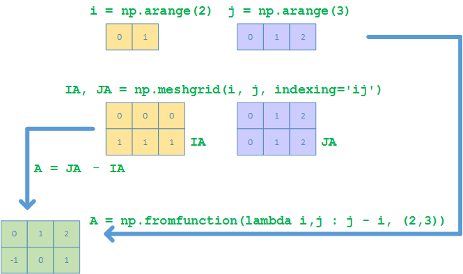
10. Meshgrids

假设要产生一个如下的meshgrid

\[ A_{ij} = j - i \]

产生meshgrids的办法，可以有以下4种（这里假定产生的矩阵大小是3x2）

The C way

>>> A = np.empty((2,3))
>>> for i in range(2):
	  for j in range(3):
		A[i,j] = j - i
>>> A
array([[ 0.,  1.,  2.],
       [-1.,  0.,  1.]])

The Python way

>>> c = [[(j-i) for j in range(3)] for i in range(2)]
>>> A = np.array(c)
>>> A
array([[ 0,  1,  2],
       [-1,  0,  1]])

The Matlab way

>>> i, j = np.arange(2), np.arange(3)
>>> ia, ja = np.meshgrid(i, j, indexing='ij')
>>> ia, ja
(array([[0, 0, 0],
       [1, 1, 1]]),
 array([[0, 1, 2],
       [0, 1, 2]]))
>>> A = ja - ia
>>> A
array([[ 0,  1,  2],
       [-1,  0,  1]])
# 或者
>>> A = np.fromfunction(lambda i,j : j - i, (2,3))
>>> A
array([[ 0.,  1.,  2.],
       [-1.,  0.,  1.]])

Meshgrid - Matlab Way

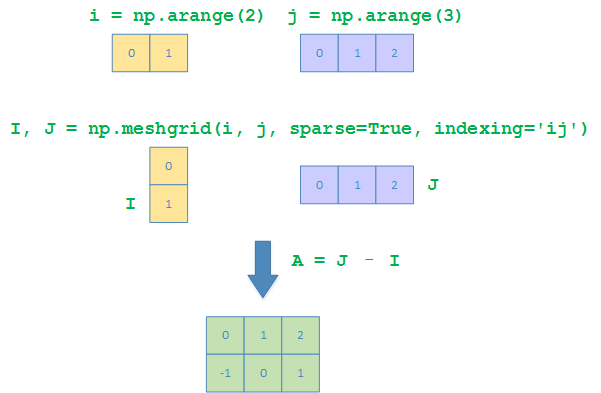
The Numpy way

>>> i, j = np.arange(2), np.arange(3)
>>> IA, JA = np.meshgrid(i, j, sparse=True, indexing='ij')
>>> IA
array([[0],
       [1]])
>>> JA
array([[0, 1, 2]])
>>> A = JA - IA
>>> A
array([[ 0,  1,  2],
       [-1,  0,  1]])

Meshgrid - Numpy way

11. Matrix Statistics

常见统计函数

函数	作用
`np.min`	最小值
`np.max`	最大值
`np.argmin`	最小值索引
`np.argmax`	最大值索引
`np.any`	至少有一个非0
`np.all`	全部非0
`np.sum`	求和
`np.std`	标准差
`np.var`	方差
`np.mean`	平均值/期望
`np.median`	平均值/期望
`np.percentile`	百分比值

各个函数都可以不加axis参数来计算所有的元素的统计值
可以加axis=0来计算沿列方向的统计值
可以加axis=1来计算沿行方向的统计值

`np.min`

>>> a = np.array([[4,8,5], [9,3,1]])
>>> np.min(a)
1
>>> np.min(a, axis=0)
array([4, 3, 1])
>>> np.min(a, axis=1)
array([4, 1])

`np.max`

>>> a = np.array([[4,8,5], [9,3,1]])
>>> np.max(a)
9
>>> np.max(a, axis=0)
array([9, 8, 5])
>>> np.max(a, axis=1)
array([8, 9])

`np.argmin`

>>> a = np.array([[4,8,5], [9,3,1]])
>>> np.argmin(a)
5
# 可以使用unravel_index来获取转换为二维的索引
>>> np.unravel_index(np.argmin(a), a.shape)
(1, 2)
>>> np.argmin(a, axis=0)
array([0, 1, 1], dtype=int64)
>>> np.argmin(a, axis=1)
array([0, 2], dtype=int64)

`np.argmax`

>>> a = np.array([[4,8,5], [9,3,1]])
>>> np.argmax(a)
3
# 可以使用unravel_index来获取转换为二维的索引
>>> np.unravel_index(np.argmax(a), a.shape)
(1, 0)
>>> np.argmax(a, axis=0)
array([1, 0, 0], dtype=int64)
>>> np.argmax(a, axis=1)
array([1, 0], dtype=int64)

`np.any`

>>> a = np.array([[4,8,5], [9,3,1]])
>>> np.any(a)
True
>>> np.any(a, axis=0)
array([ True,  True,  True])
>>> np.any(a, axis=1)
array([ True,  True])

`np.all`

>>> a = np.array([[4,8,5], [9,3,1]])
>>> np.all(a)
True
>>> np.all(a, axis=0)
array([ True,  True,  True])
>>> np.all(a, axis=1)
array([ True,  True])

`np.sum`

>>> a = np.array([[4,8,5], [9,3,1]])
>>> np.sum(a)
30
>>> np.sum(a, axis=0)
array([13, 11,  6])
>>> np.sum(a, axis=1)
array([17, 13])

`np.std`

>>> a = np.array([[4,8,5], [9,3,1]])
>>> np.std(a)
2.7688746209726918
>>> np.std(a, axis=0)
array([2.5, 2.5, 2. ])
>>> np.std(a, axis=1)
array([1.69967317, 3.39934634])

`np.var`

>>> a = np.array([[4,8,5], [9,3,1]])
>>> np.var(a)
7.666666666666667
>>> np.var(a, axis=0)
array([6.25, 6.25, 4.  ])
>>> np.var(a, axis=1)
array([ 2.88888889, 11.55555556])

`np.mean`, `np.median`

>>> a = np.array([[4,8,5], [9,3,1]])
>>> np.mean(a)
5.0
>>> np.mean(a, axis=0)
array([6.5, 5.5, 3. ])
>>> np.mean(a, axis=1)
array([5.66666667, 4.33333333])
>>> np.median(a)
4.5
>>> np.median(a, axis=0)
array([6.5, 5.5, 3. ])
>>> np.median(a, axis=1)
array([5., 3.])

`np.percentile`

>>> a = np.array([[4,8,5], [9,3,1]])
>>> np.percentile(a, 65)
5.75
>>> np.percentile(a, 65, axis=0)
array([7.25, 6.25, 3.6 ])
>>> np.percentile(a, 65, axis=1)
array([5.9, 4.8])

12. Matrix Sorting

主要的函数

函数	作用	备注
`np.argsort`	按照某列（行）排序，返回索引
`ndarray.argsort`	按照某列（行）排序，返回索引	调用对象是`ndarray`
`np.lexsort`	总是按列进行排序
`np.flipud`	对2D array按行上下翻转(up/down)
`np.fliplr`	对2D array按列左右翻转(left/right)

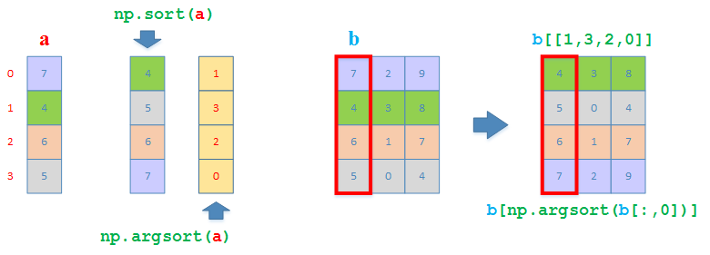
`np.argsort`

按照指定的列（行）排序，返回索引数组

实际上一个ndarray的object上也有argsort方法可以直接调用

排序一个1D array

>>> a = np.array([7, 4, 6, 5])
>>> a.argsort()
array([1, 3, 2, 0], dtype=int64)
>>> np.argsort(a)
array([1, 3, 2, 0], dtype=int64)

按照第一列排序整个2D array

>>> b = np.array([[7,2,9], [4,3,8], [6,1,7], [5,0,4]])
>>> b[np.argsort(b[:,0])]
array([[4, 3, 8],
       [5, 0, 4],
       [6, 1, 7],
       [7, 2, 9]])
# 也可以直接在新的ndarray上调用argsort，然后借用索引数组取得排序后的2D array
>>> b[b[:,0].argsort()]
array([[4, 3, 8],
       [5, 0, 4],
       [6, 1, 7],
       [7, 2, 9]])
# 效果相当于按索引返回新2D array
>>> b[[1,3,2,0]]
array([[4, 3, 8],
       [5, 0, 4],
       [6, 1, 7],
       [7, 2, 9]])

np.argsort

`np.flipud`， `np.fliplr`

np.flipud：用来将2D array上下翻转
np.fliplr：用来将2D array左右翻转

>>> a = np.array([[3, 4, 5, 6], [2, 7, 0, -1], [1, 5, 3, 18], [2, 6, 1989, 3]])
>>> a
array([[   3,    4,    5,    6],
       [   2,    7,    0,   -1],
       [   1,    5,    3,   18],
       [   2,    6, 1989,    3]])
>>> np.flipud(a)
array([[   2,    6, 1989,    3],
       [   1,    5,    3,   18],
       [   2,    7,    0,   -1],
       [   3,    4,    5,    6]])
>>> np.fliplr(a)
array([[   6,    5,    4,    3],
       [  -1,    0,    7,    2],
       [  18,    3,    5,    1],
       [   3, 1989,    6,    2]])

`np.lexsort`

np.lexsort总是把每列当做一个整体进行排序（从下到上），返回的索引数组是列的索引

>>> a = np.array([[3, 4, 5, 6], [2, 7, 0, -1], [1, 5, 3, 18], [2, 6, 1989, 3]])
>>> a
array([[   3,    4,    5,    6],
       [   2,    7,    0,   -1],
       [   1,    5,    3,   18],
       [   2,    6, 1989,    3]])
# 返回列的索引
>>> idx = np.lexsort(a)
>>> idx
array([0, 3, 1, 2], dtype=int64)
# 按照列的索引数组取得新数组，得到排序后的结果
>>> a[:,idx]
array([[   3,    6,    4,    5],
       [   2,   -1,    7,    0],
       [   1,   18,    5,    3],
       [   2,    3,    6, 1989]])   # <--- 按照2 < 3 < 6 < 1989得到的排序顺序

pandas中有更加易读的sort_values函数可以按照行/列排序

>>> a = np.array([[3, 4, 5, 6], [2, 7, 0, -1], [1, 5, 3, 18], [2, 6, 1989, 3]])
>>> a
array([[   3,    4,    5,    6],
       [   2,    7,    0,   -1],
       [   1,    5,    3,   18],
       [   2,    6, 1989,    3]])
# 先按照第0列，再按照第2列进行排序，这里axis参数默认为0（按列）
>>> pd.DataFrame(a).sort_values(by=[0,2]).to_numpy()
array([[   1,    5,    3,   18],
       [   2,    7,    0,   -1],
       [   2,    6, 1989,    3],
       [   3,    4,    5,    6]])
# 先按照第0列，再按照第2列进行排序，这里显示指定axis参数为0（按列）
>>> pd.DataFrame(a).sort_values(by=[0, 2], axis=0).to_numpy()
array([[   1,    5,    3,   18],
       [   2,    7,    0,   -1],
       [   2,    6, 1989,    3],
       [   3,    4,    5,    6]])
# 先按照第1行，再按照第3行进行排序，这里显示指定axis参数为1（按行）
>>> pd.DataFrame(a).sort_values(by=[1, 3], axis=1).to_numpy()
array([[   6,    5,    3,    4],
       [  -1,    0,    2,    7],
       [  18,    3,    1,    5],
       [   3, 1989,    2,    6]])

13. 3D and Above Matrix

用到的函数

函数	作用
`np.concatenate`	沿`axis=0\|1\|2`的方向连接
`np.moveaxis`	参数为`(a, srcAxis, destAxis)`
`np.swapaxes`
`np.einsum`

Numpy中3D array的维度顺序

在Numpy中，3D array的维度顺序是(z, y, x)，即和正常的(x, y, z)是相反的逆序。

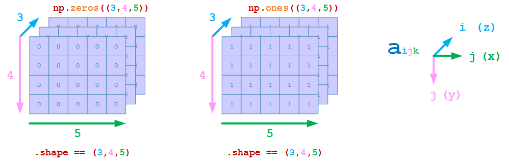
例如，创建z方向为3，y方向为4，x方向为5的3D array

>>> np.zeros((3,4,5))
array([[[0., 0., 0., 0., 0.],
        [0., 0., 0., 0., 0.],
        [0., 0., 0., 0., 0.],
        [0., 0., 0., 0., 0.]],

       [[0., 0., 0., 0., 0.],
        [0., 0., 0., 0., 0.],
        [0., 0., 0., 0., 0.],
        [0., 0., 0., 0., 0.]],

       [[0., 0., 0., 0., 0.],
        [0., 0., 0., 0., 0.],
        [0., 0., 0., 0., 0.],
        [0., 0., 0., 0., 0.]]])
>>> np.ones((3,4,5))
array([[[1., 1., 1., 1., 1.],
        [1., 1., 1., 1., 1.],
        [1., 1., 1., 1., 1.],
        [1., 1., 1., 1., 1.]],

       [[1., 1., 1., 1., 1.],
        [1., 1., 1., 1., 1.],
        [1., 1., 1., 1., 1.],
        [1., 1., 1., 1., 1.]],

       [[1., 1., 1., 1., 1.],
        [1., 1., 1., 1., 1.],
        [1., 1., 1., 1., 1.],
        [1., 1., 1., 1., 1.]]])
# 注意，np.random.ran函数的参数不是一个元组
>>> np.random.rand(3,4,5)
array([[[0.06299431, 0.09575032, 0.2670843 , 0.51132979, 0.29522357],
        [0.99386711, 0.18979029, 0.88268506, 0.8844051 , 0.3979463 ],
        [0.52145756, 0.2953166 , 0.98018492, 0.15031576, 0.35522931],
        [0.01009925, 0.93094333, 0.23642368, 0.00796226, 0.2548972 ]],

       [[0.92253603, 0.5261462 , 0.07146182, 0.06805223, 0.67127133],
        [0.14054481, 0.27912101, 0.12922132, 0.08241845, 0.78589279],
        [0.90330273, 0.32816306, 0.41328599, 0.18650637, 0.58881924],
        [0.39545397, 0.47953933, 0.25072117, 0.2345669 , 0.14524772]],

       [[0.28491979, 0.55260934, 0.19610983, 0.86477694, 0.35238863],
        [0.85913433, 0.56783708, 0.76408683, 0.11193118, 0.36949155],
        [0.36358321, 0.51957791, 0.34842336, 0.79710159, 0.58843289],
        [0.74677968, 0.44109851, 0.35527215, 0.733685  , 0.40455108]]])

`np.concatenate`

使用np.concatenate连接3D array的示意如下

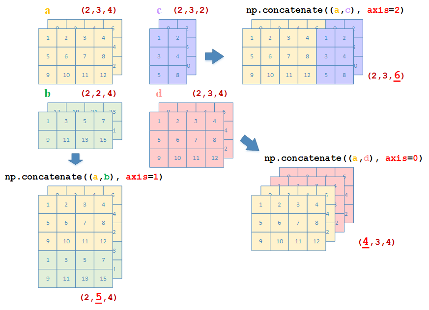
定义以下3个3D array，其中

a：a.shape = (2, 3, 4)
b：b.shape = (2, 2, 4)
c：c.shape = (2, 3, 2)
d：d.shape = (2, 3, 4)

>>> a = np.array([ [[1,2,3,4], [5,6,7,8], [9,10,11,12]], [[0,2,4,6], [8,10,12,14], [16,18,20,22]] ])
>>> a
array([[[ 1,  2,  3,  4],
        [ 5,  6,  7,  8],
        [ 9, 10, 11, 12]],

       [[ 0,  2,  4,  6],
        [ 8, 10, 12, 14],
        [16, 18, 20, 22]]])
>>> b = np.array([ [[1,3,5,7], [9,11,13,15]], [[17,19,21,23], [25,27,29,31]] ])
>>> b
array([[[ 1,  3,  5,  7],
        [ 9, 11, 13, 15]],

       [[17, 19, 21, 23],
        [25, 27, 29, 31]]])
>>> c = np.array([ [[1,2], [3,4], [5,8]], [[0,2],[4,6],[8,10]] ])
>>> d = a - 10
>>> d
array([[[ -9,  -8,  -7,  -6],
        [ -5,  -4,  -3,  -2],
        [ -1,   0,   1,   2]],

       [[-10,  -8,  -6,  -4],
        [ -2,   0,   2,   4],
        [  6,   8,  10,  12]]])
>>> a.shape
(2, 3, 4)
>>> b.shape
(2, 2, 4)
>>> c.shape
(2, 3, 2)
>>> d.shape
(2, 3, 4)

沿`z`方向连接（`axis = 0`)

>>> np.concatenate((a,d), axis=0)
array([[[  1,   2,   3,   4],
        [  5,   6,   7,   8],
        [  9,  10,  11,  12]],

       [[  0,   2,   4,   6],
        [  8,  10,  12,  14],
        [ 16,  18,  20,  22]],

       [[ -9,  -8,  -7,  -6],
        [ -5,  -4,  -3,  -2],
        [ -1,   0,   1,   2]],

       [[-10,  -8,  -6,  -4],
        [ -2,   0,   2,   4],
        [  6,   8,  10,  12]]])

沿`y`方向连接（`axis = 1`)

>>> np.concatenate((a,b), axis=1)
array([[[ 1,  2,  3,  4],
        [ 5,  6,  7,  8],
        [ 9, 10, 11, 12],
        [ 1,  3,  5,  7],
        [ 9, 11, 13, 15]],

       [[ 0,  2,  4,  6],
        [ 8, 10, 12, 14],
        [16, 18, 20, 22],
        [17, 19, 21, 23],
        [25, 27, 29, 31]]])

沿`x`方向连接（`axis = 2`)

>>> np.concatenate((a,c), axis=2)
array([[[ 1,  2,  3,  4,  1,  2],
        [ 5,  6,  7,  8,  3,  4],
        [ 9, 10, 11, 12,  5,  8]],

       [[ 0,  2,  4,  6,  0,  2],
        [ 8, 10, 12, 14,  4,  6],
        [16, 18, 20, 22,  8, 10]]])

`np.hstack`,`np.vstack`,`np.dstack`

值得注意的是，np.hstack,np.vstack,np.dstack将输入的3D array参数的三个维度分别当做(y, x, z)，而并非通常意义上的(z, y, x)

14. Summary

Related functions

Functions	Effect	Notes
`np.zeros()`
`np.empty()`
`np.full()`
`np.zeros_like()`
`np.ones_like()`
`np.empty_like()`
`np.full_like()`
`np.arange()`
`np.linspace()`
`np.random.randint()`
`np.random.rand()`
`np.random.uniform`
`np.random.default_rng().intergers()`
`np.random.default_rng().random()`
`np.random.default_rng().uniform()`
`np.where()`
`np.clip()`
`np.floor()`
`np.ceil()`
`np.round()`
`np.sqrt()`
`np.exp()`
`np.log()`
`np.dot()`	`arr @ arr`
`np.cross()`
`np.hypot()`
`np.sort()`
`arr.index()`	`arr` is `ndarry`
`np.allclose()`

NumPy Notes

NumPy Illustrated: The Visual Guide to NumPy

1. Vectors, the 1D Arrays

初始化Numpy array用到的函数

使用单调序列初始化Numpy array

创建随机数组

2. Vector indexing

基本索引操作

Boolean索引

3. Vector operations

基本操作：vector之间的加减乘除整除

基本操作：vector与scalar之间的加减乘除整除

截断近似函数

一些数学函数

基本的统计函数

排序函数

4. Searching for an element in a vector

Python list search - index method

Numpy list search

5. Comparing floats

6. Matrices, the 2D Array

基本概念

常用函数

二维数组的索引（切片slice）

7. The axis argument

轴参数（axis argument）

矩阵的算术运算

点积和叉积（内积和外积）

8. Row vectors & column vectors

9. Matrix manipulations

主要的函数

拼接和分割函数

Numpy中的拼接函数

Numpy中的分割函数

矩阵的复制

矩阵行和列的删除与插入

函数pad

10. Meshgrids

The C way

The Python way

The Matlab way

The Numpy way

11. Matrix Statistics

常见统计函数

np.min

np.max

np.argmin

np.argmax

np.any

np.all

np.sum

np.std

np.var

np.mean, np.median

np.percentile

12. Matrix Sorting

主要的函数

np.argsort

np.flipud， np.fliplr

np.lexsort

13. 3D and Above Matrix

用到的函数

Numpy中3D array的维度顺序

np.concatenate

沿z方向连接（axis = 0)

沿y方向连接（axis = 1)

沿x方向连接（axis = 2)

np.hstack,np.vstack,np.dstack

14. Summary

Related functions

函数`pad`

`np.min`

`np.max`

`np.argmin`

`np.argmax`

`np.any`

`np.all`

`np.sum`

`np.std`

`np.var`

`np.mean`, `np.median`

`np.percentile`

`np.argsort`

`np.flipud`， `np.fliplr`

`np.lexsort`

`np.concatenate`

沿`z`方向连接（`axis = 0`)

沿`y`方向连接（`axis = 1`)

沿`x`方向连接（`axis = 2`)

`np.hstack`,`np.vstack`,`np.dstack`